flowchart LR
  A{Atomic\nData} --> B[Manipulation]
  B --> D(Style)
  D --> G{Geometry\nOutput}
Fetch from the PDB
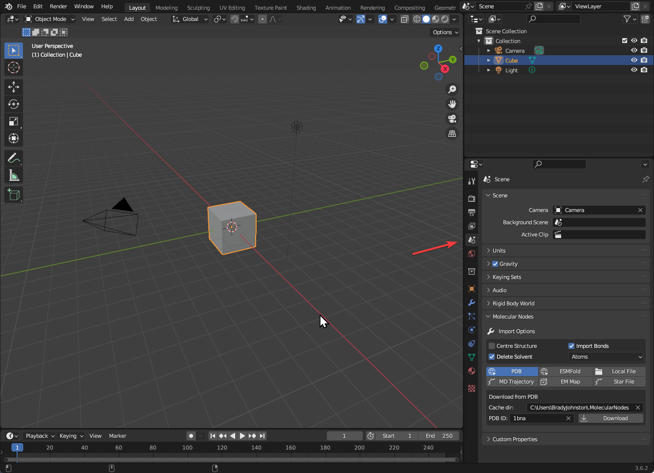
Molecules, simulations and other file formats can all be imported via the Molecular Nodes subpanel. This panel can be found under the Scene Properties panel. This is the small cone and spheres icon on the right. This contains all of the different options for importing molecular data currently available inside of Molecular Nodes.
You can download a structure directly from the PDB, just from the accession code. Molecular Nodes will download the file as a .bcif file and cache it locally on your computer, then open the file in to Blender. This is the quickest way to import structures that are already available via the wwPDB. Currently this downloads via the RCSB.
To download directly from the PDB, you can use the PDB tab.
PDB Tab
In this tab you can input the PDB ID to be used for downloading the structure. You can also change where Molecular Nodes caches the downloaded structures. By default it will be in a hidden .MolecularNodes folder in your home directory.
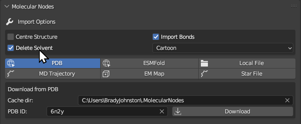
Type in the code, choose your import options such as starting style, and click download. The new object will appear in the outliner. It will appear inside of the MolecularNodes collection and should have the name of the PDB ID used to fetch the structure. If an object already exists with that name, it will be appended with a .001 or similar suffix.
The molecule may appear inside of the default cube, so you may have to delete it before the protein becomes visible.
4OZS from the PDBEdit Mode
The protein is imported as a 3D mesh, with a vertex for each atom and an edge for each bond. What you are seeing is the result of passing that data through a geometry-processing pipeline. The underlying data is still available, and you can even look at it (and edit it if you wish) by going using edit mode with Tab
You are editing the underlying atomic data, not the cartoon itself. The cartoon is rebuilt on top of the edited atomic data, which is why part of it also moves with the atoms when they are moved.
It is probably ill-advised to manually edit the atomic data by hand, but it is important to understand the structure of the data inside of Blender & Molecular Nodes.
Rendered Views
While the molecule is imported, we are in 3D view by default. We can change to a rendered view to view the molecule with more accurately calculated lighting effects.
Changing Styles
The protein is now imported in the scene. To change the way the protein is displayed, we have to use the Geometry Nodes editor. This is where we change the nodes that are use to process the underlying atomic data, resulting in the final 3D object we can see in front of us.
To access Geometry Nodes panel, we can either select the Geoemtry Nodes workspace, or split the current viewport and change one of the workspaces into the node editor.
You can change the workspace through the tabs in the top of Blender. You can split workspaces by hovering over the corner of a workspace, and then clicking and dragging. You can merge to workspaces by clicking and dragging from one into another, while dragging into the same workspace will split it and create two workspaces.
Geometry node trees are explained more in the next section.
In short, the atomic data comes through the Group Input on the left, and the final 3D model goes out the Group Output to the right. Each node in between performs some actions on the data. The first node changes the colours of the atoms. The last node applies the given style. When importing we chose the Cartoon style default, so we have a cartoon node.
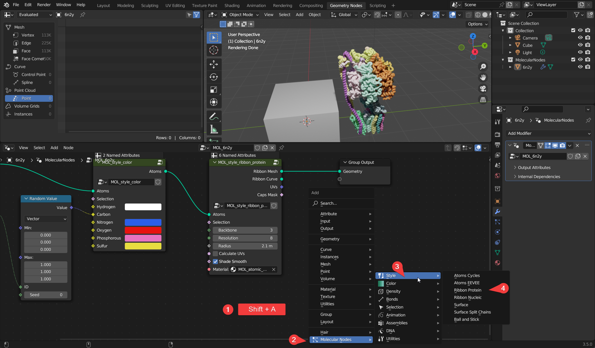
We can add a new node through the Add menu, or we can use Shift + A to add new nodes. We can click and drag on the noodle outputs and inputs to remove and create new connections. Notice how when the complete ‘circuit’ or ‘flow diagram’ goes through the ball and stick node, the style changes to ball and stick. When it flows through the cartoon node, the style changes to cartoon.
Geometry Nodes Editor
This is where we edit the node graph for Molecular Nodes. The node graph is a geometry processing program you create, that is read and executed by Blender from left to right. Each node performs an action on the geometry that is passed into it, and the result of that action is passed out to the right. Think of it as creating a set of rules for the computer to follow. You define the rules, and the computer can follow those same rules, even if you start with a different data set.
The data flows like a river, along the green noodles of the node graph. There must be only 1 final output. If you are using the molecular data, then there must also be a single input.

The data flows from left to right, like water through a river.
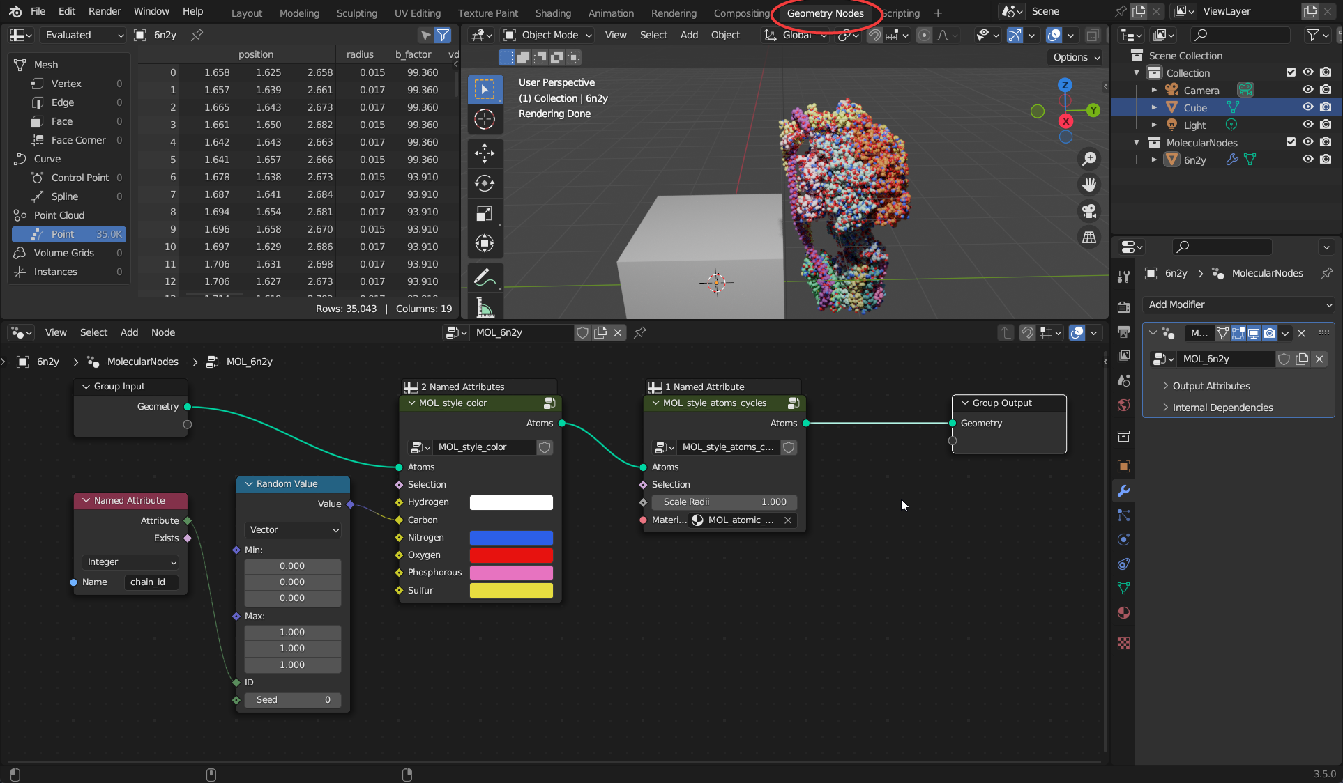
The starting style MOL_style_atoms_cycles is only visible via inside of the Cycles render engine. You can add other styles manipulate the data through other nodes, by adding them with Shift + A and navigating to the MolecularNodes panel at the bottom. There are several categories of nodes for different animations and styles. You can add the Ribbon Protein node, which will create a ribbon representation based on the alpha carbons in the structure. If there is not colour in the structure, ensure that the node has a material MOL_atomic_material at the bottom of the node.
The data flows through the node graph from left to right. There should always be one input, which is the atomic data that is stored in the 3D mesh of the atoms and bonds. There should also be only one output, which is the final geometry that has been created throughout the node graph.
flowchart LR
  A{Atomic\nData} --> B[Manipulation]

  B --> D(Style 1)
  B --> E(Style 2)
  B --> S(Style 3)

  sS[Selection] --> S

  E --> F[Join\nGeometry]
  D --> F
  S --> F

  F --> G{Geometry\nOutput}
As demonstrated in the diagram, the flow of the data can split across multiple different branches of the tree, with the result of each parallel computation being combined before being exported.
Each of these different branches can be a different style, in this example shown two different styles are applied, and the third style has a custom selection. All of the styles are the result of the same data manipulation.
The node graph in between can be as complex as you want to make it, as long as there is a continuous connection to the output of the geometry, it should produce a result.
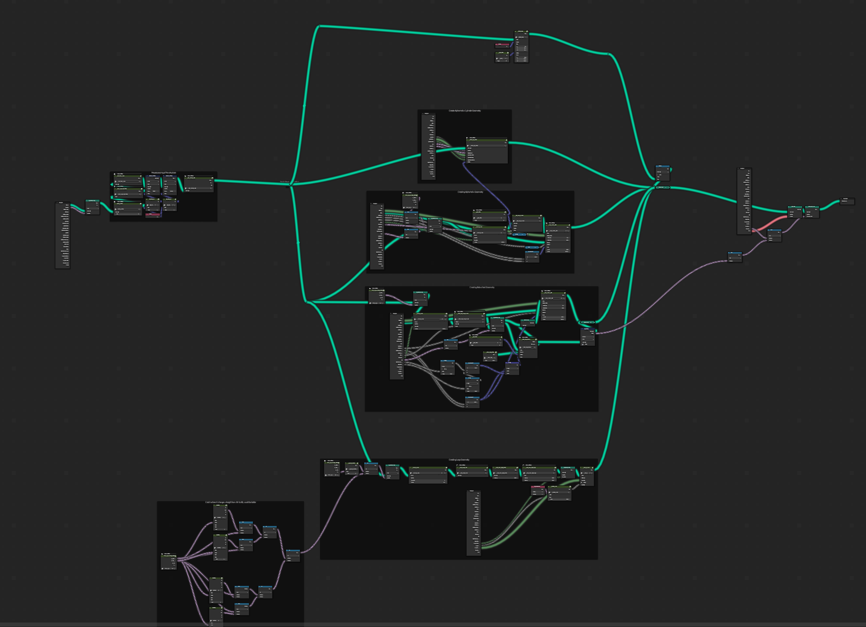
Combining multiple different nodes you can create protein models and complex 3D scenes. In the example below, there is a node tree which should be present on every new structure imported via MolecularNodes. The atoms and bonds are passed in from the left, the atoms are given a colour based on their element and their chain_id, and then the atoms are styled as atoms, scaling the atom radii to 1.00.
The data flows through the node tree from left to right, along the bright green lines. The atomic data comes in, goes through layers of manipulation, a style is applied, and the created geometry is then outputted from the node tree.
Editing the Styles
To change how each style looks, you can edit the default values of the nodes. By changing the values, you change the numbers that are used in the creation of the 3D models. The style will only change if it is being output through the node tree. You can click and drag to change the values smoothly. You can hold Shift while dragging the values to change them more accurately.
Combining Styles
To complete this tutorial, we will combine the use of Selection and Join Geometry to create a style which shows the side chains as ball and stick while also showing the cartoon style.
The style should usually be the last node that you apply to a model. You can’t apply a style after another style, as the output of a style is 3D geometry and not ‘atom-like’ geometry. Instead, we can combine two styles with a Join Geometry node. That way, we create both styles in parallel and then join them together before outputting them all through the Group Output node.
The node can be found under Geometry or by going through the search for Join Geometry
Selections
Many nodes will have a Selection input, which you can’t manually edit. This input is a Boolean attribute and says whether or not to apply an operation to atoms based on if the value is True or False.
You can use selections via the Molecular Nodes -> Selection menu. In this example we use the Backbone node to select atoms based on if they are part of the backbone, the side chain, or just alpha carbons.
You can see as we connect different outputs from the Backbone node, we get different results in the final style.